Deep learning noter – Convolutional Neural Networks 8 & 11/10 2021

Last time:

• Key-ideas to exploited
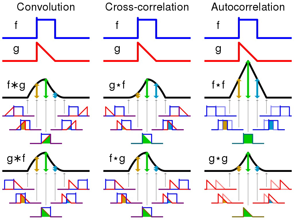
• Convolution
• Visual explanations of conolution
• In convolution the entire input is used and manipulated by a kernel in chunks
• From a input string, an matrix is created
• 2d image manipulation example

Covolution

Instead of learning full matrix, only a couple of weights of the kernel is needed to be learned.

Weights are repeated (the same).

It looks like a feed forward network.

With sparse connectivity inputs are only influences the activation of the layers its connected to in the next layer. This means chaning the input, might not yield influential changes in the next layer, in comparinson to using the entire matrix. Although it will have larger influence in future layers.

Parameter sharing:

• Parameter sharing refers to reusing the same parameters for multiple functions in a model.
• It’s very efficient.

Depths of the outcome volume

Detpth of the output colume is a hyerparameter. The set of neurons that are in the same reguin of the input is defined as input depth.

Multiple kernels

Multiple kernels works in multiplication as defined (w^t)*x+h. The images do not need to match any sizes for multiple kernels to work. It can however get enificient.

Image –> Low level features –> Mid-level features –> High-level features — Lineraly seprable classifier –> …

Absence of equvariance

The method is not equivariant.

To have argumented data, images need to be rotated, zoomed and manipulated manually.

Pooling

With pooling we empathise the need for the input image for low level features, and that it is no longer needed when working with high-level features.

Pooling modifes the output to a smaller dimension.

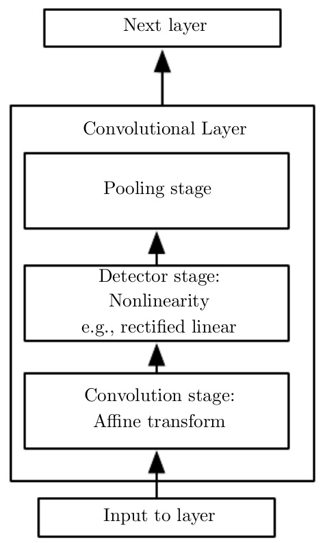
Stages in deep learning:

1. Conolution
2. Detector
3. Pooling

A classic aritecure:

The types of pooling functions:

• Max pooling – which reports the maximum putput within a retangular neighborhood
• Average of a retangular neighborhood
• L^2 norm of a retangular neighborhood
• Weighted average pooling – whis is based on the distane form the cetral pixel

Pooling should/could be used to:

• Max pooling: shifted values slightly, and reduced size of output value.
• Increases resiliance towards other translations. For this spacial manipulation is used.
• Pooling with down samlpling summarizes the responses of a whole neighboorhood. This makes it posible tp use more detector units than pooling units.

VVG / VVG Net

VGG is a convolutional network model. Diverstions to the model are common.

Vgg is used for very deep convolutional networks for large scale image recognition.

From keras it can be chosen if convolutional netork, all or both should be used.

Variants of Convolution

• strided convolution – similar to pooling
• Local connections – features are not repeated as often, but local features is the focus.
• Convolution
• Full connections

Initialiazation

• Random initialization – based on random kernels the output is trained. This is done multiple times, and the best initilization is used for training.
• No training
  • Random initialiazation
  • Edge detection
  • Unsupervised criterion
• Bluring filter
• Sharpen

Convolution in Keras

Defining Convolutions in Keras

# Defining Convolutions in Keras
from keras import layers
from keras import models

model = models.Sequential()
model.add(layers.Conv2D(32, (3, 3), activation='relu',
input_shape=(28, 28, 1)))
model.add(layers.MaxPooling2D((2, 2)))
model.add(layers.Conv2D(64, (3, 3), activation='relu'))
model.add(layers.MaxPooling2D((2, 2)))
model.add(layers.Conv2D(64, (3, 3), activation='relu’))

model.add(layers.Flatten())
model.add(layers.Dense(64, activation='relu'))
model.add(layers.Dense(10, activation='softmax'))

The Convolutional Layer in Keras

# The Convolutional Layer in Keras
keras.layers.Conv2D(filters, kernel_size, #Number of filters, kernel dimensions
    strides=(1, 1), # Using a stride?
    padding='valid’, # ‘valid’ means only valid positions are used.
    ‘same’ means output has same dimension as input
    data_format=None, # ‘channels_last’ or ‘channels_first’
    dilation_rate=(1, 1), # Increase the field of “vision”
    activation=None, # Rest of the parameters same as dense layer
    use_bias=True,
    kernel_initializer='glorot_uniform’,
    bias_initializer='zeros’,
    kernel_regularizer=None,
    bias_regularizer=None,
    activity_regularizer=None,
    kernel_constraint=None,
    bias_constraint=None
)

The Pooling Layer in Keras

# The Pooling Layer in Keras
keras.layers.MaxPooling2D(
    pool_size=(2, 2), # Size of the pooling
    strides=None, # Integer, tuple of 2 integers, or None. Strides
    values. If None, it will default to pool_size.
    padding='valid’, # One of "valid" or "same"
    data_format=None # Same as with Conv2D
)

Training your Model

# Training your Model
history = model.fit_generator(
    train_generator,
    steps_per_epoch=100,
    epochs=30,
    validation_data=validation_generator,
    validation_steps=50
)

Automatically Distort Images

# Automatically Distort Images
datagen = ImageDataGenerator(
    rotation_range=40,
    width_shift_range=0.2,
    height_shift_range=0.2,
    shear_range=0.2,
    zoom_range=0.2,
    horizontal_flip=True,
    fill_mode='nearest’
)

Visualize Activations

from keras.models import Model
layer_outputs = [layer.output for layer in model.layers]
activation_model = Model(inputs=model.input, outputs=layer_outputs)
activations = activation_model.predict(X_train[10].reshape(1,28,28,1))

def display_activation(activations, col_s, row_s, act_index):
    activation = activations[act_index]
    activation_index=0
    fig, ax = plt.subplots(row_size, col_size, figsize=(row_s2.5,col_s1.5))
    for row in range(0,row_size):
        for col in range(0,col_size):
            ax[row][col].imshow(activation[0, :, :, activation_index], cmap='gray')
            activation_index += 1

Activation filters

It’s a small kernel. It’s more intresting to look at previous levels that already modified the input.

For images comparable to constructing adversarial examples can be created. This is done by using any grey scale image and calculate the overall activation of the filter of interest. If maximization of the peak of this particular filter is performed computation of the gradient with respect to the input and adaptation of the out/input image to maximize overall activation of the filter can be performed.

The more layers are used, the more complex and colourfully diverse the filters will be.